
Project Quantum Shield · Simulation note
When a cultural barrier starts to show up in the genome
A thousand generations of two small populations, drifting apart at the rate their contact allows.
What the script actually does
Take two small populations of the same species. Every generation three things happen to them. A few genes flip by mutation. A few individuals move between the groups. And then the next generation is drawn by chance from the ones who are there — which, in a small population, is the loudest of the three effects.
Run that loop a thousand times over a hundred independent positions in the genome, and measure how different the two groups have become. That measure is FST: zero if the groups are interchangeable, one if they share nothing at the positions being watched.
The single knob is contact. Cultural polarization is entered as a barrier coefficient C, and its only job is to shrink the migration term: me = m0 × (1 − C). Nothing in the model knows what the barrier is made of — language, geography, politics, taste. It only knows how much traffic gets through.
The mutation rate is where the quantum thread enters. Instead of a generic textbook value, the script uses μ = 1.73 × 10⁻⁴, the occupancy figure from the tautomer work in Notebook 1. That is the only place the two halves of the project touch numerically, and it is a modeled number, not a measured one.
The parameters in plain terms
Effective population size — N_e = 30 per deme
How many individuals actually pass genes forward. Small numbers make chance matter more.
Baseline migration — m_0 = 0.05
The fraction of each group that would exchange with the other in an open, unpolarized world.
Cultural barrier coefficient — C = 0.00 – 0.99
How much polarization closes that exchange. Effective migration is m_e = m_0 × (1 − C).
Mutation rate — μ = 1.73 × 10⁻⁴
Taken from the modeled tautomer occupancy of the G*–C* pair — the quantum term entering a classical population model.
Differentiation index — F_ST = 0 – 1
0 means the two groups are genetically indistinguishable; 1 means they share nothing at the sampled loci.
What came out of this run
| C | m_e | F_ST ≥ 0.50 | F_ST ≥ 0.75 | F_ST at gen 1000 |
|---|---|---|---|---|
| 0.00 | 0.0500 | never | never | 0.04 |
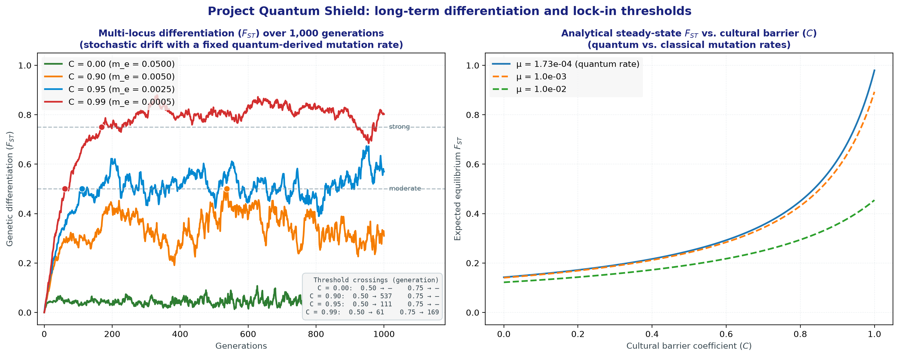
| 0.90 | 0.0050 | gen 537 | never | 0.31 |
| 0.95 | 0.0025 | gen 111 | never | 0.57 |
| 0.99 | 0.0005 | gen 61 | gen 169 | 0.80 |
The shape of the result is not gradual. At C = 0, five percent exchange per generation is enough to hold the two groups together indefinitely — the green trace never leaves the floor. At C = 0.90 the groups drift apart but wander below the halfway line for centuries. At C = 0.99, with one in two thousand crossing over, the halfway line is passed in sixty-one generations and the upper line inside two hundred.
That is the finding worth sitting with: the interesting behaviour is compressed into the last percent of closure. Almost-closed and closed are different regimes, not different degrees.
The right panel says the same thing without the noise. Wright's approximation is flat and unremarkable across most of the range, then turns sharply upward as C approaches one — and the choice of mutation rate barely matters until migration has already nearly stopped. Mutation is not the driver here. Isolation is. The quantum rate matters for what kind of variation appears, not for how fast the groups separate.
What this is not
- Not a human forecast. N_e = 30 is a toy population. Real human effective sizes are orders of magnitude larger, which slows drift enormously. The model shows a mechanism's shape, not a timetable.
- Not speciation. F_ST measures allele-frequency differentiation. The 0.50 and 0.75 lines are conventional reading marks, not reproductive-isolation thresholds. Nothing here says two populations can no longer interbreed.
- One seed, one run. Every trajectory above is a single stochastic realization at seed 42. The crossing generations would move under a different seed; the ordering across C values would not.
- The falsifier is measurable. If observed F_ST between strongly separated human populations stays flat while measured assortative contact drops toward zero, the barrier-to-migration mapping at the heart of this script is wrong.
The script
Runs in a few seconds with NumPy and Matplotlib. It is also in the Project Quantum Shield repository as cultural_isolation_v2.py.
# ==============================================================================# Wright's F-statistics with quantum mutation: long-term differentiation# Project Quantum Shield — supplementary materials, v2# =============================================================================="""Multi-locus Wright-Fisher model of two subpopulations (demes) under geneticdrift, restricted migration (m_e), and a constant mutation rate (mu) taken fromthe modeled G*-C* tautomer occupancy. Cultural polarization enters as a barriercoefficient C that scales effective migration: m_e = m_0 * (1 - C).Output: a dual-panel figure.1) 1,000-generation stochastic F_ST trajectories for C = 0.00 ... 0.99, withthe generations at which F_ST first crosses 0.50 and 0.75.2) Analytical steady-state F_ST vs. C for three mutation rates, including thequantum tautomeric rate mu = 1.73e-4."""import numpy as npimport matplotlibmatplotlib.use("Agg")import matplotlib.pyplot as pltdef run_simulation(N_e=30, m_0=0.05, generations=1000, num_loci=100, mu=1.73e-4,out_path="cultural-isolation-simulation-v2.png"):C_values = [0.0, 0.90, 0.95, 0.99]np.random.seed(42)fst_history = np.zeros((len(C_values), generations + 1))for c_idx, C in enumerate(C_values):m_e = m_0 * (1.0 - C)p1 = np.full(num_loci, 0.5)p2 = np.full(num_loci, 0.5)def fst(p1, p2):p_mean = (p1 + p2) / 2.0H_T = np.sum(2 * p_mean * (1 - p_mean))H_S = np.sum(p1 * (1 - p1) + p2 * (1 - p2))return (H_T - H_S) / H_T if H_T > 0 else 1.0fst_history[c_idx, 0] = fst(p1, p2)for gen in range(1, generations + 1):# 1. mutation (symmetric, rate mu)p1_mut = p1 * (1 - mu) + (1 - p1) * mup2_mut = p2 * (1 - mu) + (1 - p2) * mu# 2. migration between demesp1_mig = p1_mut * (1 - m_e) + p2_mut * m_ep2_mig = p2_mut * (1 - m_e) + p1_mut * m_e# 3. Wright-Fisher drift (binomial sampling per locus)p1 = np.random.binomial(2 * N_e, p1_mig) / (2 * N_e)p2 = np.random.binomial(2 * N_e, p2_mig) / (2 * N_e)fst_history[c_idx, gen] = fst(p1, p2)# first crossing of each thresholdcrossings = {}for c_idx, C in enumerate(C_values):crossings[C] = {}for th in (0.50, 0.75):hit = np.where(fst_history[c_idx] >= th)[0]crossings[C][th] = int(hit[0]) if len(hit) else Nonefig, (ax1, ax2) = plt.subplots(1, 2, figsize=(15, 6))for c_idx, C in enumerate(C_values):ax1.plot(range(generations + 1), fst_history[c_idx], linewidth=2,label=f"C = {C:.2f} (m_e = {m_0 * (1 - C):.4f})")for th in (0.50, 0.75):t = crossings[C][th]if t is not None:ax1.scatter(t, th, s=55, zorder=5, edgecolor="white", linewidth=0.8)ax1.axhline(0.50, color="#78909c", linestyle="--", linewidth=1.2, alpha=0.6)ax1.axhline(0.75, color="#78909c", linestyle="--", linewidth=1.2, alpha=0.6)ax1.set_xlabel("Generations")ax1.set_ylabel("Genetic differentiation ($F_{ST}$)")ax1.set_ylim(-0.05, 1.05)ax1.legend(loc="upper left")C_fine = np.linspace(0.0, 1.0, 500)for mu_val in [1.73e-4, 1e-3, 1e-2]:m_e_fine = m_0 * (1.0 - C_fine)# Wright's approximation with migration and mutation:# F_ST ~= 1 / (1 + 4 * N_e * (m_e + mu))fst_steady = 1.0 / (1.0 + 4.0 * N_e * (m_e_fine + mu_val))ax2.plot(C_fine, fst_steady, linewidth=2,linestyle="-" if mu_val == 1.73e-4 else "--",label=f"mu = {mu_val:.2e}")ax2.set_xlabel("Cultural barrier coefficient ($C$)")ax2.set_ylabel("Expected equilibrium $F_{ST}$")ax2.set_ylim(-0.05, 1.05)ax2.legend(loc="upper left")plt.tight_layout()plt.savefig(out_path, dpi=200, bbox_inches="tight")plt.close()print(crossings)if __name__ == "__main__":run_simulation()