LC Circuits and the Geometry of Radiation

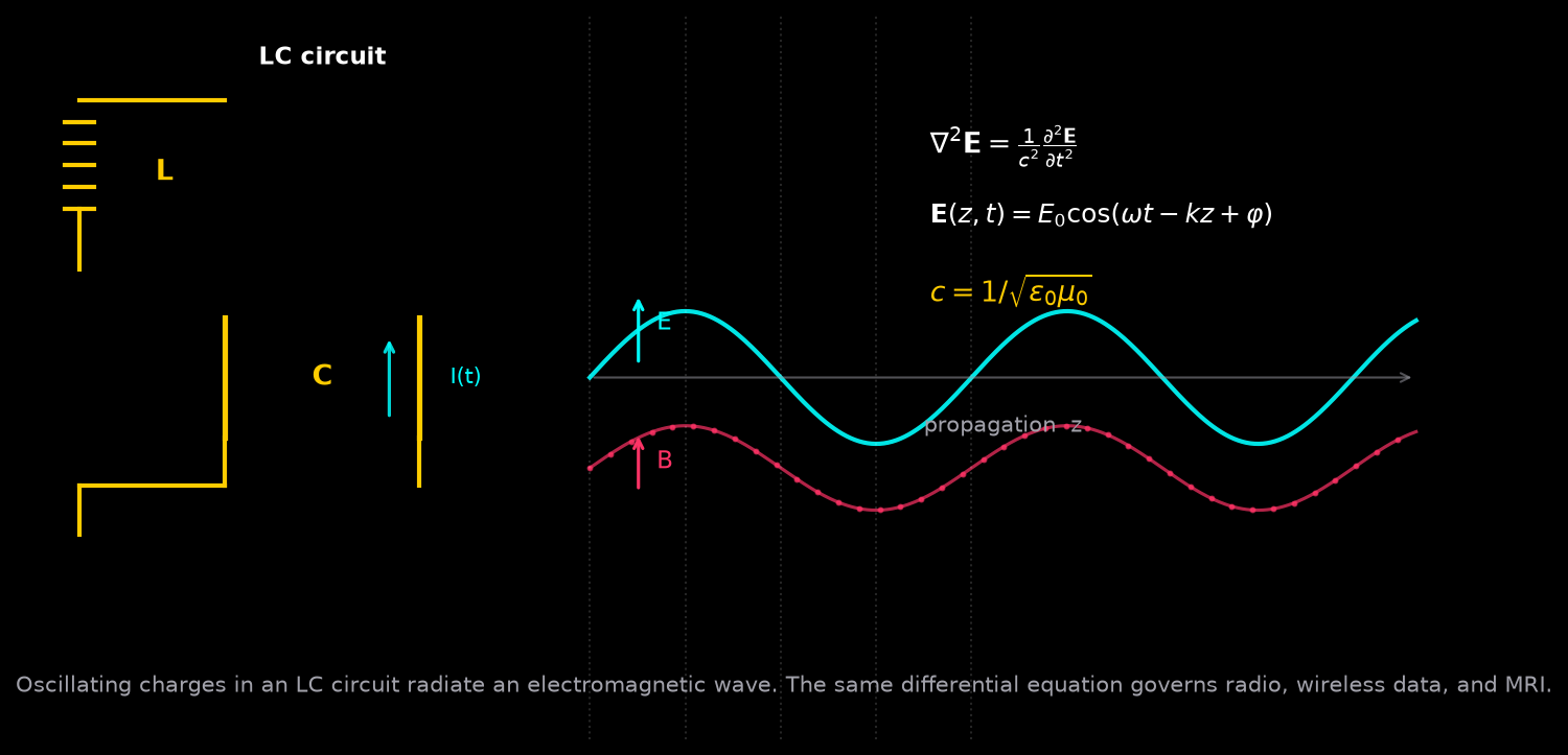
The Mathematica post that prompted this figure is doing something quietly radical: it shows a single differential equation underwriting three apparently separate technologies. The wave equation

does not care whether the medium is a classroom blackboard, a radio antenna, or the receiver coils of an MRI machine. What changes is the boundary condition: the geometry of the circuit, the shape of the antenna, the permeability and permittivity of tissue. The equation stays the same.

The speed c = 1/√(ε₀μ₀) is not a coincidence extracted from Maxwell’s equations; it is the conversion factor between the electric and magnetic constants of empty space. In matter the same relation becomes c/√(ε_rμ_r), because the medium itself participates in the geometry.

This is Gaia to Geometry in miniature: a Riemannian or differential-geometric structure (here the flat wave operator) is borrowed to describe a local phenomenon, while the full geometry of the situation — the circuit, the antenna, the body — supplies the boundary conditions. The equation is the passport, not the prison.

Turn the knobs

The static figure hides which parts of the picture are the equation and which are the boundary conditions. Move the controls below and the difference becomes visible: capacitance and inductance set the resonance, resistance sets how long the circuit rings before the energy is gone, and the wave speed in the medium sets the wavelength for a given frequency. The wave equation never changes.

Two things are worth watching for. Push the damping high enough and the circuit stops oscillating altogether — the readouts drop to overdamped, and there is nothing left to radiate. And note that L and C only ever appear as their product in the resonance and as their ratio in the impedance: two knobs, but the frequency responds to one combination and the matching to another.

The same wave as a spiral

The flat snapshot above is only one choice of drawing. If the two transverse components are given equal amplitude and a quarter-cycle phase offset — circular polarisation — the field vector does not oscillate in a plane, it rotates as the wave advances. Its tip then traces a helix wound around the direction of travel, one full turn per wavelength.

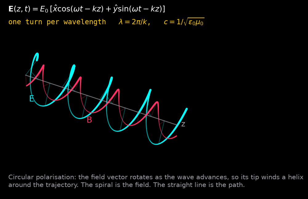
Two things are worth keeping separate here. The spiral is the field, not the path: nothing travels along the helix. The energy moves straight down the central trajectory while the orientation of the field winds around it. And the winding is not decoration — the number of turns per wavelength is fixed, and the handedness (left or right circular) is a discrete label the wave carries with it. Linear polarisation is the degenerate case where the helix collapses into a plane.

That distinction — a straight trajectory carrying a wound structure — is the honest version of the braid figure. A single circularly polarised beam is one thread with a twist, which is a helix, not yet a braid; braiding needs more than one thread, or the azimuthal phase winding of an optical vortex, where the topological charge becomes an integer that cannot be changed continuously.

And the same wave as a braid

So give it more threads. Three circularly polarised strands sharing one axis, each offset by a third of a cycle, project onto the page as a standard three-strand braid. Nothing has been drawn by hand: the transverse position of strand n is y_n(z) = R sin(kz + 2πn/3), and the sign of its radial component decides which strand passes in front at each meeting. The crossings are the phase offsets.

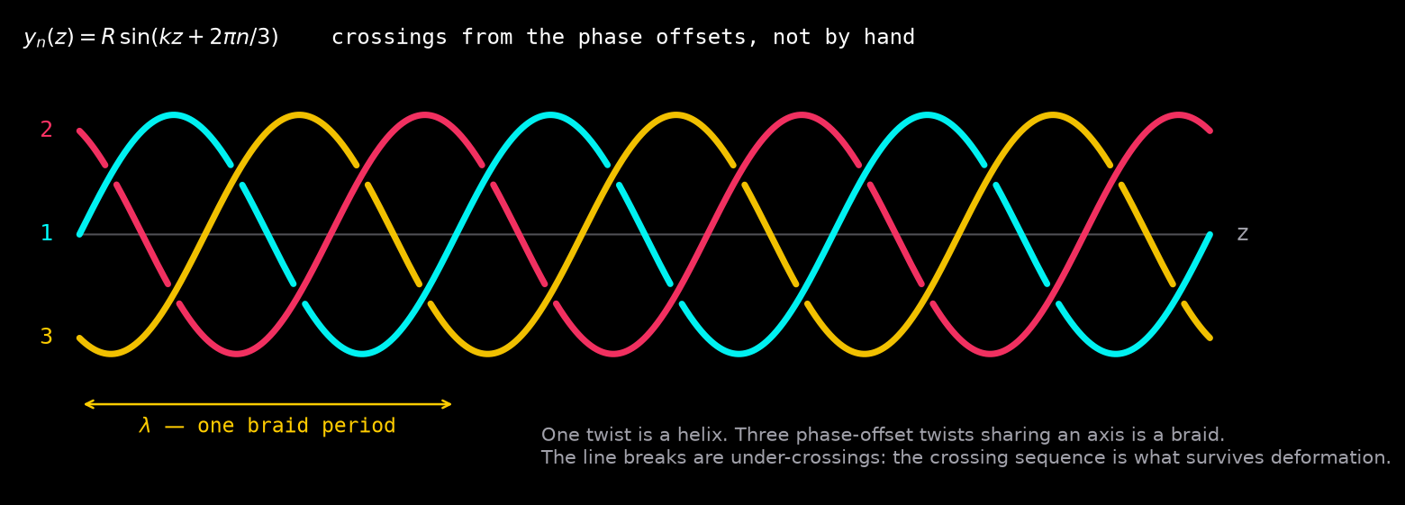
What the picture makes available is a different kind of quantity. The helix gave us a continuous phase and a handedness. The braid gives us a word: a finite sequence of crossings, each one over or under, read left to right along the axis. Stretch the strands, bend the axis, change the amplitude — the word does not change. Only cutting a strand or forcing a crossing to reverse changes it. That is the sense in which the braid carries information the geometry cannot smooth away.

Two registers to keep apart, as always. Three independent beams superposed in vacuum do not physically braid; they pass through one another, because Maxwell’s equations are linear. What braids here is the arrangement — the pattern of relative position, which is real and measurable, and which returns to itself once per wavelength. Genuine topological locking needs something more: a nonlinear medium, a guiding structure, or the phase singularities of vortex beams, where the crossings are pinned rather than merely traced. The diagram is a passport for that idea, not a proof of it.

Why this matters for the project

The post is a reminder that “energy as incoming information” is not only a philosophical move. In an LC circuit, the energy stored in the capacitor’s electric field and the inductor’s magnetic field is converted into a propagating wave whose phase, amplitude, and polarization carry information. The geometry of the medium selects which information arrives.

For Volume 27, this is a clean example of a borrowed geometry: Maxwell’s equations and the wave equation are not the territory, but they are a reliable map for a large class of territories. The falsifier is equally clean: find a circuit or antenna where the wave equation predicts the wrong propagation, and the boundary conditions — not the equation — will be where the correction lives.